3 Sampling distributions and confidence intervals

3.1 Random and stratified sampling

A simple random sample gives each eligible observation an equal chance of selection. Stratified sampling divides the population into predefined groups and samples within each group. If sampling fractions differ across strata, population estimates may require sampling weights.

simple_60 <- dat |> slice_sample(n=60)
stratified_60 <- dat |> group_by(treatment_arm) |> slice_sample(n=20) |> ungroup()

table(simple_60$treatment_arm)
#> 
#> Control  Drug_A  Drug_B 
#>      24      20      16
table(stratified_60$treatment_arm)
#> 
#> Control  Drug_A  Drug_B 
#>      20      20      20

3.2 Sampling bias

Bias occurs when the sampling process systematically produces a sample that does not represent the target population. For example, sampling only older participants may give distorted estimates if the target population includes all ages.

tibble(
  sample=c("All participants","Age ≥65 years"),
  mean_age=c(mean(dat$age_years), mean(dat$age_years[dat$age_years>=65])),
  mean_sbp=c(mean(dat$sbp_baseline_mmHg), mean(dat$sbp_baseline_mmHg[dat$age_years>=65]))
) |>
  kbl(digits=2, caption="A deliberately biased sampling example")

3.3 Sampling distribution and standard error

The sampling distribution describes how a statistic would vary across repeated samples. Its standard deviation is the standard error (SE).

For the sample mean,

\[ SE(\bar X)=\frac{\sigma}{\sqrt n}. \]

Because the population standard deviation \(\sigma\) is usually unknown, the SE is estimated using the sample standard deviation:

\[ \widehat{SE}(\bar X)=\frac{s}{\sqrt n}. \]

3.3.1 Repeated-sampling simulation

The observed baseline SBP values are treated as an empirical population, and samples of 40 observations are repeatedly drawn with replacement.

sbp <- na.omit(dat$sbp_baseline_mmHg)
means40 <- replicate(3000, mean(sample(sbp, 40, replace=TRUE)))

tibble(
  empirical_mean=mean(means40),
  empirical_SE=sd(means40),
  theoretical_SE=sd(sbp)/sqrt(40)
) |>
  kbl(digits=3, caption="Sampling distribution of the mean")

Table 3.2: Sampling distribution of the mean

empirical_mean	empirical_SE	theoretical_SE
130.1	2.146	2.126

ggplot(tibble(mean_sbp=means40), aes(mean_sbp)) +
  geom_histogram(bins=35, fill="#547D8E", colour="white") +
  labs(x="Sample mean SBP (mmHg)", y="Simulation count")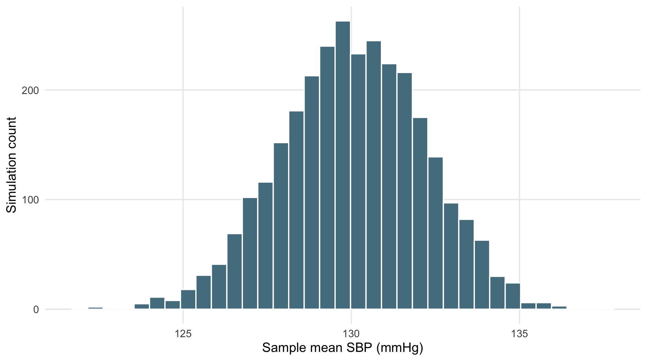

Figure 3.1: Simulated sampling distribution of mean baseline SBP for samples of size 40.

3.4 Central limit theorem

The central limit theorem (CLT) explains why the sampling distribution of a mean becomes approximately normal as sample size increases, even when the original observations are skewed. It does not imply that the original data become normal.

crp <- na.omit(dat$crp_baseline_mg_L)

clt <- bind_rows(
  tibble(value=replicate(2000, mean(sample(crp,5,TRUE))), n="n = 5"),
  tibble(value=replicate(2000, mean(sample(crp,30,TRUE))), n="n = 30"),
  tibble(value=replicate(2000, mean(sample(crp,100,TRUE))), n="n = 100")
)

ggplot(clt, aes(value)) +
  geom_histogram(bins=32, fill="#315B74", colour="white") +
  facet_wrap(~n, scales="free") +
  labs(x="Sample mean CRP (mg/L)", y="Simulation count")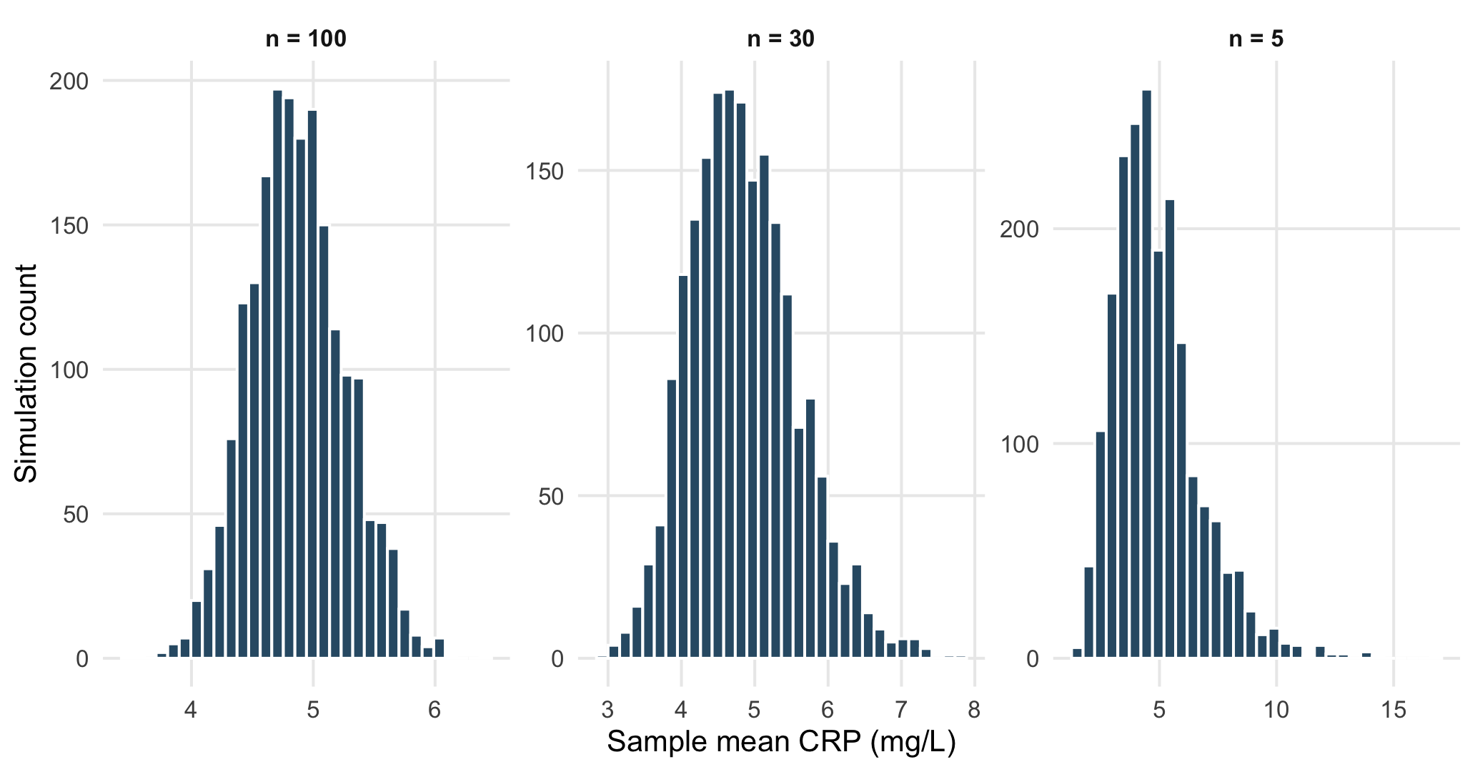

Figure 3.2: Sampling distributions of the mean for a right-skewed CRP variable.

As \(n\) increases, the sampling distribution becomes narrower and more symmetric.

3.5 Confidence intervals

A confidence interval gives a range of plausible values for the population mean. When the population variance is unknown, the sample standard deviation \(s\) is used and the interval is based on the \(t\)-distribution.

\[ \bar{x}\pm t_{1-\alpha/2,\,n-1}\frac{s}{\sqrt n}. \]

The critical value t is the multiplier taken from the \(t\)-distribution; It determines how many standard errors are used in the confidence interval, and it depends on the sample size.

t.test(dat$sbp_baseline_mmHg, conf.level=.95)$conf.int
#> [1] 128.7 131.5
#> attr(,"conf.level")
#> [1] 0.95