2.1 Measures of location
2.1.1 Mean, median, and trimmed mean
For observations \(x_1,\ldots,x_n\), the arithmetic mean is
\[ \bar{x}=\frac{1}{n}\sum_{i=1}^{n}x_i. \]
It uses every observation and is efficient for many regular distributions, but it can be strongly influenced by a long tail or extreme values. The median is the middle ordered value and is more resistant to outliers. A trimmed mean compromises between the two by removing a fixed proportion from each tail before averaging.
2.1.1.1 Arithmetic and robust location summaries
x <- dat$crp_baseline_mg_L
location <- tibble(mean=mean(x, na.rm=TRUE),
                   median=median(x, na.rm=TRUE),
                   trimmed_mean_10pct=mean(x, trim=.10, na.rm=TRUE),
                   q25=quantile(x,.25,na.rm=TRUE), q75=quantile(x,.75,na.rm=TRUE));

kbl(location, digits=2, caption="Location summaries for baseline CRP")| mean | median | trimmed_mean_10pct | q25 | q75 |
|---|---|---|---|---|
| 4.86 | 3.48 | 4.18 | 2.35 | 6.01 |
2.1.2 Weighted means
When observations carry legitimate representation or precision weights, the weighted mean is
\[ \bar{x}_w=\frac{\sum_i w_i x_i}{\sum_i w_i}. \]
The workbook contains sampling_weight specifically for sampling demonstrations.However, the trial’s primary treatment comparisons are not weighted by this educational variable.
2.1.2.1 Weighted mean for systolic blood pressure
ok <- complete.cases(dat$sbp_baseline_mmHg, dat$sampling_weight)

tibble(unweighted=mean(dat$sbp_baseline_mmHg[ok]),
       weighted=weighted.mean(dat$sbp_baseline_mmHg[ok], dat$sampling_weight[ok])) |>
kbl(digits=2, caption="Unweighted and weighted baseline SBP")| unweighted | weighted |
|---|---|
| 130.1 | 130.2 |
2.2 Measures of variability
2.2.1 SD, IQR, and MAD
The sample variance measures the average squared spread of observations around the sample mean.
\[ s^2=\frac{\sum_{i=1}^{n}(x_i-\bar{x})^2}{n-1}, \]
and the sample standard deviation is
\[ s=\sqrt{s^2}, \]
which returns dispersion to the original measurement scale.
The interquartile range is
\[ IQR=Q_3-Q_1, \]
the width of the middle 50% of observations.
The median absolute deviation (MAD) measures the typical distance of observations from the median.
\[ MAD=\operatorname{median}_{i}\left|x_i-\tilde{x}\right|, \]
where \(\tilde{x}\) is the sample median. MAD is a robust measure of dispersion because it is based on absolute deviations from the median and is less sensitive to extreme observations than the standard deviation.
2.2.1.1 Measures of spread and dispersion
tibble(
  variable = c("Baseline SBP", "Baseline CRP"),
  SD = c(
    sd(dat$sbp_baseline_mmHg, na.rm=TRUE),
    sd(dat$crp_baseline_mg_L, na.rm=TRUE)
  ),
  IQR = c(
    IQR(dat$sbp_baseline_mmHg, na.rm=TRUE),
    IQR(dat$crp_baseline_mg_L, na.rm=TRUE)
  ),
  MAD_scaled = c(
    mad(dat$sbp_baseline_mmHg, na.rm=TRUE),
    mad(dat$crp_baseline_mg_L, na.rm=TRUE)
  ),
  MAD_raw = c(
    mad(dat$sbp_baseline_mmHg, constant=1, na.rm=TRUE),
    mad(dat$crp_baseline_mg_L, constant=1, na.rm=TRUE)
  )
) |>
kbl(digits=2, caption="Classical and robust measures of spread")| variable | SD | IQR | MAD_scaled | MAD_raw |
|---|---|---|---|---|
| Baseline SBP | 13.44 | 16.42 | 12.53 | 8.45 |
| Baseline CRP | 4.06 | 3.66 | 2.31 | 1.56 |
2.2.2 Raw versus scaled MAD
The distinction is important. The lecture formula is the raw median absolute deviation. R’s mad() multiplies that quantity by a consistency constant by default; mad(x, constant=1) reproduces the raw formula.
2.3 Percentiles and distributional summaries
A percentile is a cut point in the ordered data: the \(p\)th quantile is a value at or below which approximately \(100p\%\) of observations fall. Percentiles are especially useful for skewed biomarkers and for identifying clinically relevant distribution tails.
2.4 Grouped descriptive statistics
A good descriptive table reports the number of non-missing observations and summaries appropriate to the distribution. SBP is reasonably summarized by mean and SD; CRP is long-tailed, so median and IQR are more informative.
2.4.1 Summary by randomized arm
grouped <- dat |>
  group_by(treatment_arm) |>
  summarise(
    n=n(),
    across(c(age_years, sbp_baseline_mmHg),
           list(mean=~mean(.x,na.rm=TRUE), sd=~sd(.x,na.rm=TRUE)),
           .names="{.fn}_{.col}"),
    across(c(crp_baseline_mg_L, biomarker_baseline_ng_mL),
           list(median=~median(.x,na.rm=TRUE), IQR=~IQR(.x,na.rm=TRUE)),
           .names="{.fn}_{.col}"),
    .groups="drop"
  )

kbl(grouped, digits=2, caption="Selected baseline summaries by randomized arm")| treatment_arm | n | mean_age_years | sd_age_years | mean_sbp_baseline_mmHg | sd_sbp_baseline_mmHg | median_crp_baseline_mg_L | IQR_crp_baseline_mg_L | median_biomarker_baseline_ng_mL | IQR_biomarker_baseline_ng_mL |
|---|---|---|---|---|---|---|---|---|---|
| Control | 120 | 52.42 | 13.45 | 129.5 | 13.74 | 3.40 | 3.85 | 95.3 | 56.62 |
| Drug_A | 120 | 55.88 | 12.50 | 129.1 | 13.48 | 3.71 | 3.55 | 96.3 | 54.93 |
| Drug_B | 120 | 56.79 | 11.50 | 131.6 | 13.09 | 3.44 | 3.41 | 101.8 | 59.15 |
In a randomized trial, baseline tables describe the sample. Routine p-values are usually unnecessary because baseline differences arise by chance from randomization.
2.5 Categorical data
For categorical variables, frequencies and proportions are the natural summaries.
2.5.1 Frequencies and proportions
severity <- dat |> count(treatment_arm, baseline_severity, name="n") |>
                  group_by(treatment_arm) |>
                  mutate(percent=100*n/sum(n)) |> ungroup()

kbl(severity, digits=1, caption="Baseline severity by treatment arm")| treatment_arm | baseline_severity | n | percent |
|---|---|---|---|
| Control | Mild | 45 | 37.5 |
| Control | Moderate | 33 | 27.5 |
| Control | Severe | 42 | 35.0 |
| Drug_A | Mild | 32 | 26.7 |
| Drug_A | Moderate | 56 | 46.7 |
| Drug_A | Severe | 32 | 26.7 |
| Drug_B | Mild | 34 | 28.3 |
| Drug_B | Moderate | 48 | 40.0 |
| Drug_B | Severe | 38 | 31.7 |
2.5.1.1 Clinical-response proportions
response_tab <- table(dat$treatment_arm, dat$response);
response_tab;
#>
#>           No Yes
#>   Control 88  32
#>   Drug_A  68  52
#>   Drug_B  50  70
prop.table(response_tab, margin=1)
#>
#>               No    Yes
#>   Control 0.7333 0.2667
#>   Drug_A  0.5667 0.4333
#>   Drug_B  0.4167 0.5833
Row proportions provide an initial indication of association between two categorical variables: differences across treatment arms may suggest an association between treatment type and clinical response.
The corresponding inferential analysis is developed in Chapters 3 and 6.
2.6 Histograms, density plots, and boxplots
A histogram is a visual frequency table; its appearance depends on bin width.
A kernel density plot smooths the empirical distribution and uses density, not raw count or a direct category proportion, on the vertical axis. Its scale is defined so that the total area under the density curve is 1.
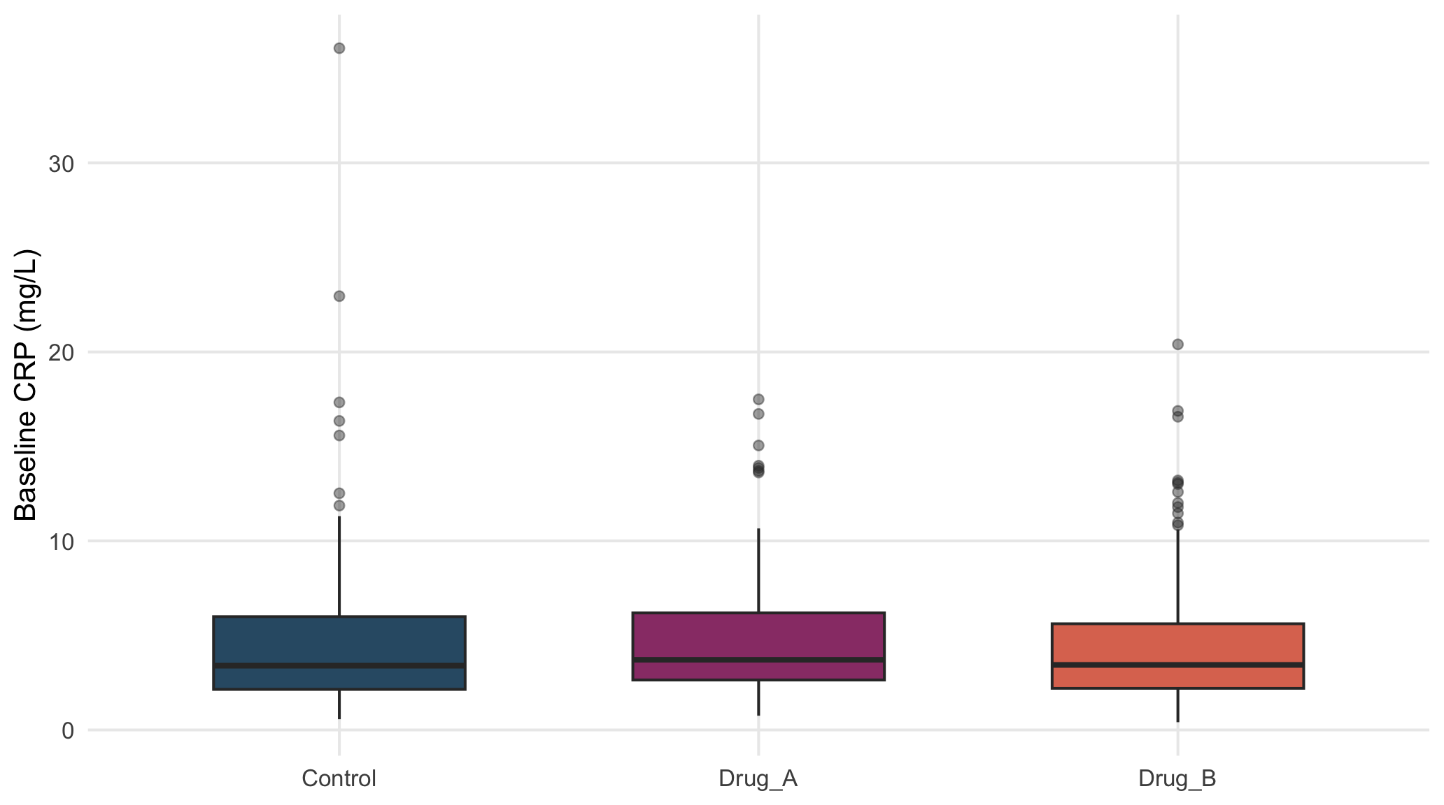
A boxplot compactly displays the median, quartiles, and points beyond the conventional whiskers.
2.6.1 Distribution shape
base_long <- dat |>
        dplyr::select(treatment_arm, sbp_baseline_mmHg, crp_baseline_mg_L, biomarker_baseline_ng_mL, qol_baseline_0_100) |>
        pivot_longer(-treatment_arm, names_to="measure", values_to="value")

ggplot(base_long, aes(value, fill=treatment_arm)) +
  geom_histogram(bins=28, alpha=.55, position="identity", na.rm=TRUE) +
  facet_wrap(~measure, scales="free", ncol=2) +
  scale_fill_manual(values=pal) +
  labs(x=NULL, y="Count", fill="Treatment")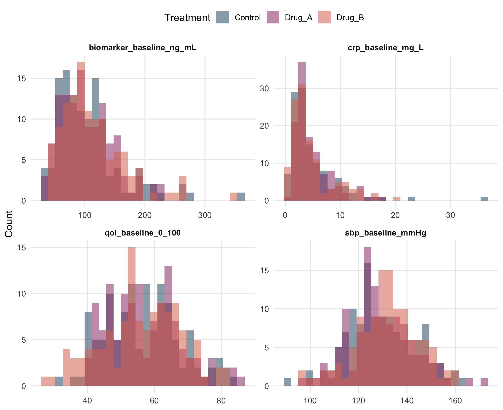
Figure 2.1: selected baseline distributions by randomized treatment arm.
2.7 Outliers: observations to understand, not delete automatically
A boxplot point beyond 1.5 IQR is not automatically an erroneous observation/ outlier. Before exclusion, ask whether the value is impossible, caused by a measurement or entry error, inconsistent with source data, or simply a legitimate extreme value.
Deleting a genuine observation because it weakens significance is unacceptable.
Robust summaries, transformations, and sensitivity analyses are preferable when extreme but valid observations materially affect a model.
2.8 EDA checklist
Before inferential analysis, the analyst should be able to state: - the observational unit and whether observations are independent, paired, clustered, or repeated; - the outcome type and clinically meaningful direction of effect; - treatment/reference categories and factor coding; - the amount and pattern of missingness; - plausible ranges and units; - distributional shape, outliers, and group-specific spread; - whether a transformation has a scientific interpretation; - which baseline variables are genuinely pre-treatment covariates; - which variables are post-randomization and therefore require caution in causal treatment models.
For example, the adherence to treatment percentageadherence_pctis measured after randomization and may itself be affected by treatment. Adjusting for it can therefore change the treatment-effect estimand and introduce bias. For this reason, it is excluded from the primary treatment-effect models and considered only in clearly labeled associational analyses.