Correlation measures the strength and direction of association between two continuous variables.
| Method | Measures | Useful when |
|---|---|---|
| Pearson | linear association | the relationship is approximately linear without influential outliers |
| Spearman | monotonic rank association | data are skewed, contain outliers, or the relationship is not strictly linear |
15.1 Pearson correlation
Pearson’s correlation coefficient measures the strength and direction of a linear relationship:
\[ r=\frac{\sum_i(x_i-\bar{x})(y_i-\bar{y})} {\sqrt{\sum_i(x_i-\bar{x})^2\sum_i(y_i-\bar{y})^2}}. \]
It ranges from \(-1\) to \(1\). Values closer to \(-1\) or \(1\) indicate stronger linear association.
cor.test(~biomarker_baseline_ng_mL+biomarker_week12_ng_mL,
         data=dat,method="pearson")
#>
#>  Pearson's product-moment correlation
#>
#> data:  biomarker_baseline_ng_mL and biomarker_week12_ng_mL
#> t = 52, df = 347, p-value <0.0000000000000002
#> alternative hypothesis: true correlation is not equal to 0
#> 95 percent confidence interval:
#>  0.9286 0.9526
#> sample estimates:
#>    cor
#> 0.9418
A scatterplot should accompany Pearson correlation to assess the form of the relationship and identify influential observations.
ggplot(dat,aes(biomarker_baseline_ng_mL,biomarker_week12_ng_mL,colour=treatment_arm)) +
  geom_point(alpha=.45,na.rm=TRUE) +
  geom_smooth(method="lm",se=FALSE,na.rm=TRUE) +
  scale_colour_manual(values=pal) +
  labs(x="Baseline biomarker (ng/mL)",y="Week-12 biomarker (ng/mL)",colour="Treatment")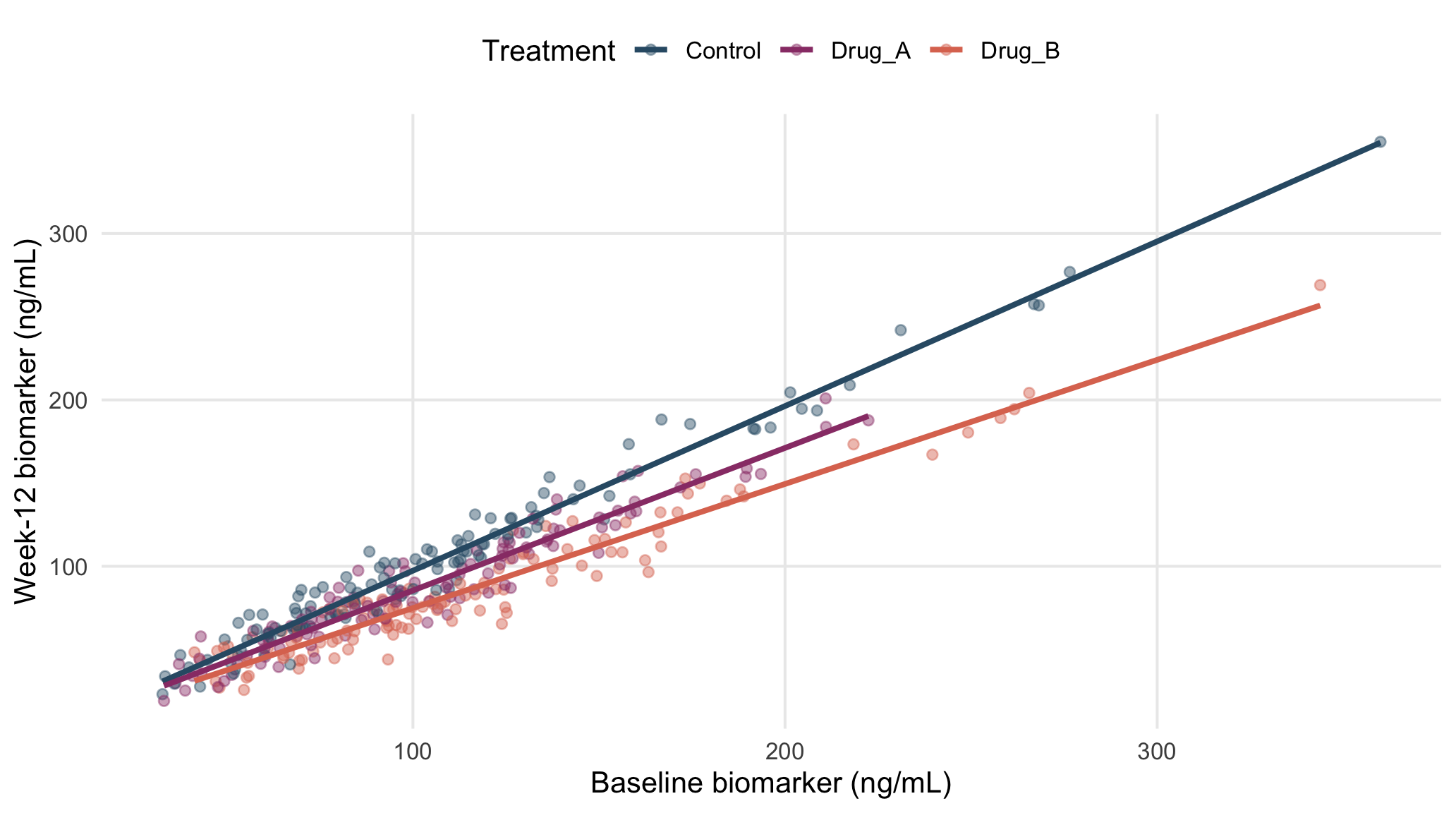
Figure 15.1: Baseline and week-12 biomarker with a linear fit.
15.2 Spearman rank correlation
Spearman correlation uses the ranks of the observations rather than their original values. It measures the strength and direction of a monotonic relationship and is useful for skewed data.
Because CRP is strongly right-skewed, Spearman correlation is appropriate for describing the association between baseline and week-12 CRP.
cor.test(~crp_baseline_mg_L+crp_week12_mg_L,
         data=dat,method="spearman",exact=FALSE)
#>
#>  Spearman's rank correlation rho
#>
#> data:  crp_baseline_mg_L and crp_week12_mg_L
#> S = 264568, p-value <0.0000000000000002
#> alternative hypothesis: true rho is not equal to 0
#> sample estimates:
#>    rho
#> 0.9582
A strong Pearson or Spearman correlation does not imply that two measurements agree, nor does it establish causation.
15.3 Correlation matrix
A correlation matrix summarizes associations among several continuous variables. Here, Spearman correlations are used because some variables are skewed.
cor_vars <- dat |> transmute(
  Age=age_years,BMI=bmi_kg_m2,`Baseline SBP`=sbp_baseline_mmHg,
  HbA1c=hba1c_pct,LDL=ldl_mg_dL,HDL=hdl_mg_dL,eGFR=egfr_mL_min_1_73m2,
  `Baseline CRP`=crp_baseline_mg_L,
  `Baseline biomarker`=biomarker_baseline_ng_mL,
  `Baseline QoL`=qol_baseline_0_100)

cm <- cor(cor_vars,use="pairwise.complete.obs",method="spearman")
round(cm,2)
#>                      Age   BMI Baseline SBP HbA1c   LDL   HDL  eGFR Baseline CRP Baseline biomarker Baseline QoL
#> Age                 1.00  0.06         0.35  0.24  0.03 -0.02 -0.76         0.15               0.13        -0.32
#> BMI                 0.06  1.00         0.28  0.30  0.01 -0.10 -0.04         0.04               0.12        -0.21
#> Baseline SBP        0.35  0.28         1.00  0.20  0.08 -0.05 -0.21         0.02               0.13        -0.20
#> HbA1c               0.24  0.30         0.20  1.00  0.07  0.03 -0.21         0.00               0.09        -0.13
#> LDL                 0.03  0.01         0.08  0.07  1.00 -0.01  0.01        -0.09              -0.03        -0.01
#> HDL                -0.02 -0.10        -0.05  0.03 -0.01  1.00  0.00        -0.06              -0.04         0.10
#> eGFR               -0.76 -0.04        -0.21 -0.21  0.01  0.00  1.00        -0.11              -0.07         0.26
#> Baseline CRP        0.15  0.04         0.02  0.00 -0.09 -0.06 -0.11         1.00               0.07        -0.19
#> Baseline biomarker  0.13  0.12         0.13  0.09 -0.03 -0.04 -0.07         0.07               1.00        -0.14
#> Baseline QoL       -0.32 -0.21        -0.20 -0.13 -0.01  0.10  0.26        -0.19              -0.14         1.00
cm_long <- as.data.frame(cm) |>
tibble::rownames_to_column("x") |>
pivot_longer(-x,names_to="y",values_to="rho")
ggplot(cm_long,aes(x,y,fill=rho)) +
geom_tile(colour="white",linewidth=.4) +
geom_text(aes(label=sprintf("%.2f",rho)),size=3) +
scale_fill_gradient2(low="#B45252",mid="white",high="#3F7F8D",limits=c(-1,1)) +
coord_equal() +
labs(x=NULL,y=NULL,fill="Spearman ρ") +
theme(axis.text.x=element_text(angle=45,hjust=1))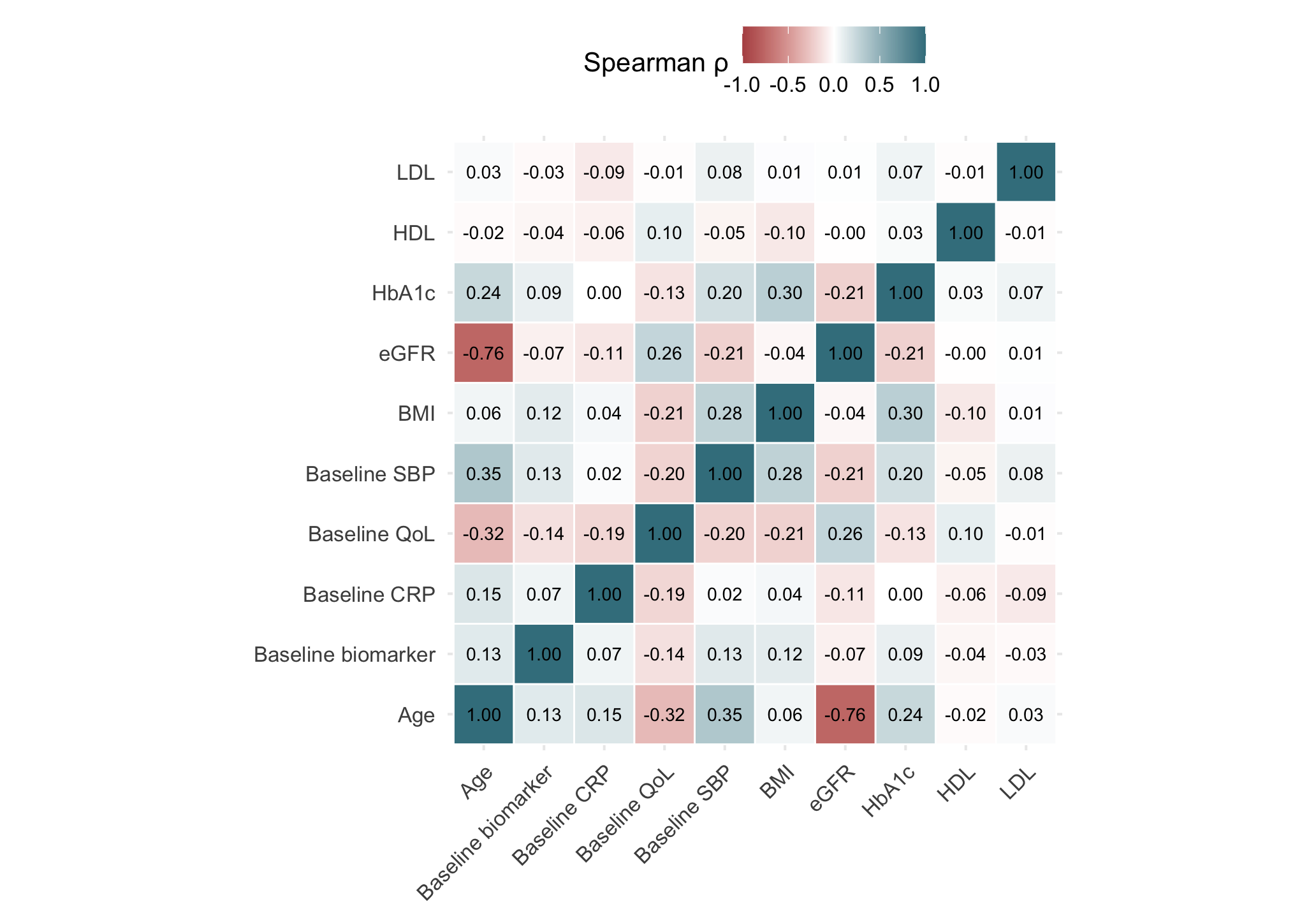
Figure 15.2: Spearman correlation matrix for selected baseline variables.
15.4 Correlation is not causation
Correlation shows whether two variables move together, but it does not show that one causes the other.
A strong correlation between baseline and follow-up measurements may indicate that baseline is useful to include in a regression model. However, the treatment effect is estimated by the regression model, not by the correlation coefficient.