ANOVA and regression are two expressions of the same linear-model framework. ANOVA is most convenient when explanatory variables are categorical; regression notation becomes more natural when continuous covariates, interactions, and adjustment are central. The key statistical object is the model, not the function name used to fit it.
13.1 One-way ANOVA
For \(k\) independent groups, one-way ANOVA tests whether all group means are equal:
\[ H_0:\mu_1=\mu_2=\cdots=\mu_k. \]
ANOVA separates the total variation into:
- Between-group variation: differences among the group means.
- Within-group variation: variation among individuals within each group.
Each source of variation is converted to a mean square (MS):
\[ MS_{\text{between}}=\frac{SS_{\text{between}}}{df_{\text{between}}}, \qquad MS_{\text{within}}=\frac{SS_{\text{within}}}{df_{\text{within}}}. \]
The F statistic is
\[ F=\frac{MS_{\text{between}}}{MS_{\text{within}}}. \]
A large \(F\) means that the group means differ more than would be expected from the variation within the groups.
13.1.1 Example: SBP change across three treatment arms
Change-score ANOVA is used here because it gives a clean demonstration of the classical one-way model. The preferred treatment-effect analysis for week-12 SBP is baseline-adjusted ANCOVA discussed later.
13.1.1.1 Group summaries for systolic blood pressure
sbp_cc <- dat |> drop_na(sbp_change)
sbp_cc |> group_by(treatment_arm) |>
          summarise(n=n(), mean=mean(sbp_change), sd=sd(sbp_change), median=median(sbp_change), .groups="drop") |>
kbl(digits=2, caption="SBP change by treatment arm")| treatment_arm | n | mean | sd | median |
|---|---|---|---|---|
| Control | 118 | -0.85 | 7.62 | -0.80 |
| Drug_A | 117 | -5.68 | 8.62 | -6.30 |
| Drug_B | 118 | -9.78 | 7.70 | -10.15 |
13.1.1.2 Distribution of systolic blood pressure by arm
ggplot(sbp_cc, aes(treatment_arm, sbp_change, fill=treatment_arm)) +
  geom_boxplot(width=.6, outlier.alpha=.35) +
  scale_fill_manual(values=pal, guide="none") +
  geom_hline(yintercept=0, linetype=2) +
  labs(x=NULL, y="SBP change (mmHg)")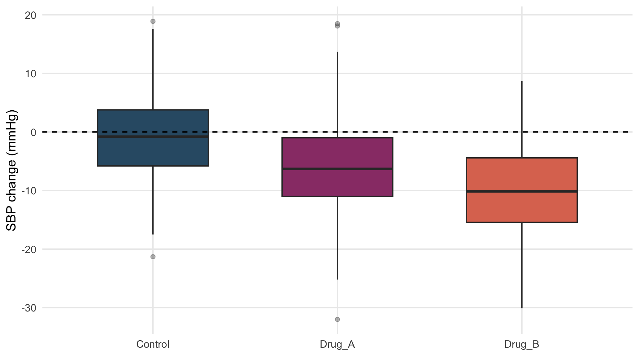
Figure 13.1: Distribution of week-12 minus baseline SBP by treatment arm.
13.1.2 Assumptions and diagnostics
The main assumptions of classical ANOVA are:
- observations are independent.
- residuals are approximately normal.
- variability is similar across groups.
Independence is determined by the study design. Normality and equal variance are assessed using residual plots and comparisons of group spread.
13.1.2.1 One-way linear-model specification
sbp_aov <- aov(sbp_change~treatment_arm, data=sbp_cc);
summary(sbp_aov);
#>                Df Sum Sq Mean Sq F value             Pr(>F)
#> treatment_arm   2   4709    2355    36.9 0.0000000000000029 ***
#> Residuals     350  22340      64
#> ---
#> Signif. codes:  0 '***' 0.001 '**' 0.01 '*' 0.05 '.' 0.1 ' ' 1

car::leveneTest(sbp_change~treatment_arm, sbp_cc, center=median)
#> Levene's Test for Homogeneity of Variance (center = median)
#>        Df F value Pr(>F)
#> group   2    0.58   0.56
#>       350
13.1.2.2 Residual and variance diagnostics
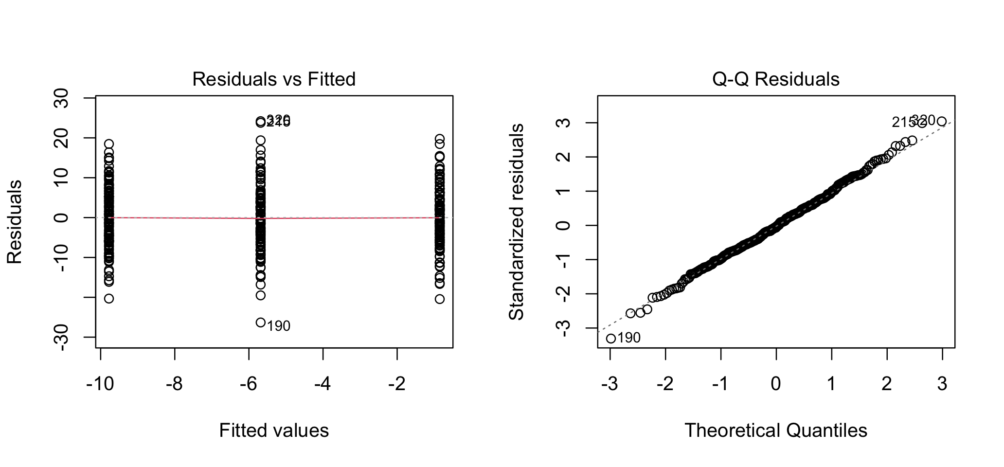
Figure 13.2: Residual diagnostics for the one-way SBP change model.
With balanced groups of roughly 120 participants, the F test is fairly robust to modest non-normality. What would be more concerning is a combination of severe skew/outliers, very unequal variances, and strongly unequal sample sizes.
13.1.3 Effect size
effectsize::eta_squared(sbp_aov, partial=FALSE)
#> # Effect Size for ANOVA (Type I)
#>
#> Parameter     | Eta2 |       95% CI
#> -----------------------------------
#> treatment_arm | 0.17 | [0.12, 1.00]
#>
#> - One-sided CIs: upper bound fixed at [1.00].
Eta-squared (\(\eta^2\)) measures the overall effect size, while post hoc tests identify which treatment groups differ from each other. Treatment-specific mean differences show how large those differences are. Here, \(\eta^2=0.17\), meaning that about 17% of the variation in SBP change is associated with treatment group.
13.1.4 Tukey HSD pairwise comparisons
If ANOVA assumptions are met, we use Tukey’s HSD for all pairwise group comparisons. It controls the family-wise error rate and reports adjusted p-values with simultaneous 95% confidence intervals.
13.1.4.1 Tukey-adjusted pairwise mean contrasts
TukeyHSD(sbp_aov)
#>   Tukey multiple comparisons of means
#>     95% family-wise confidence level
#>
#> Fit: aov(formula = sbp_change ~ treatment_arm, data = sbp_cc)
#>
#> $treatment_arm
#>                  diff     lwr    upr  p adj
#> Drug_A-Control -4.831  -7.285 -2.378 0.0000
#> Drug_B-Control -8.924 -11.372 -6.476 0.0000
#> Drug_B-Drug_A  -4.093  -6.546 -1.639 0.0003
13.2 Welch ANOVA for unequal variances
13.2.1 Preserve the mean estimand
A large variance difference does not force the question to change from means to ranks. If the scientific estimand remains the difference in means, Welch ANOVA is designed for unequal group variances.
The biomarker change scores have visibly different spreads across treatment arms.
13.2.1.1 Biomarker-change summaries
bio_change_cc <- dat |> drop_na(biomarker_change)

bio_change_cc |> group_by(treatment_arm) |>
summarise(n=n(), mean=mean(biomarker_change), sd=sd(biomarker_change), median=median(biomarker_change), .groups="drop") |> kbl(digits=2, caption="Biomarker change by treatment arm")| treatment_arm | n | mean | sd | median |
|---|---|---|---|---|
| Control | 118 | -2.71 | 9.68 | -4.25 |
| Drug_A | 116 | -14.94 | 11.93 | -14.25 |
| Drug_B | 115 | -28.73 | 17.41 | -27.60 |
13.2.2 Games–Howell follow-up
For pairwise follow-up under unequal variances, Games–Howell is more coherent than Tukey HSD because it does not impose a common variance.
13.2.2.1 Games–Howell pairwise comparisons
rstatix::games_howell_test(bio_change_cc, biomarker_change~treatment_arm) |>
          dplyr::select(group1, group2, estimate, conf.low, conf.high, p.adj) |>
kbl(digits=3, caption="Games–Howell pairwise comparisons for biomarker change")| group1 | group2 | estimate | conf.low | conf.high | p.adj |
|---|---|---|---|---|---|
| Control | Drug_A | -12.23 | -15.58 | -8.873 | 0 |
| Control | Drug_B | -26.01 | -30.39 | -21.635 | 0 |
| Drug_A | Drug_B | -13.79 | -18.43 | -9.144 | 0 |
This chapter uses Welch ANOVA to compare mean biomarker change across treatment groups. Later, a more appropriate model adjusts for baseline biomarker and includes a baseline-by-treatment interaction, because the treatment effect depends on the baseline biomarker level.
13.3 Kruskal–Wallis test for a rank-based comparison across multiple groups
13.3.1 A deliberately rank-based question
CRP change is strongly skewed and not approximately normally distributed. When the goal is to compare the groups using a rank-based method rather than compare arithmetic means, the Kruskal–Wallis test is appropriate.
13.3.1.1 CRP summaries for a rank-based question
crp_change_cc <- dat |> drop_na(crp_change)
crp_change_cc |> group_by(treatment_arm) |>
                 summarise(n=n(), median=median(crp_change), IQR=IQR(crp_change), mean=mean(crp_change), .groups="drop") |>
kbl(digits=2, caption="CRP change by treatment arm")| treatment_arm | n | median | IQR | mean |
|---|---|---|---|---|
| Control | 113 | -0.05 | 0.88 | -0.03 |
| Drug_A | 111 | -0.35 | 0.90 | -0.49 |
| Drug_B | 112 | -0.68 | 1.17 | -0.93 |
13.3.1.2 Kruskal–Wallis test and post hoc comparisons
kruskal.test(crp_change~treatment_arm, data=crp_change_cc)
#>
#>  Kruskal-Wallis rank sum test
#>
#> data:  crp_change by treatment_arm
#> Kruskal-Wallis chi-squared = 45, df = 2, p-value = 0.0000000002

# Post Hoc Test
rstatix::dunn_test(crp_change_cc, crp_change~treatment_arm, p.adjust.method="holm") |>
        dplyr::select(group1, group2, statistic, p, p.adj) |>
kbl(digits=4, caption="Dunn pairwise comparisons with Holm adjustment")| group1 | group2 | statistic | p | p.adj |
|---|---|---|---|---|
| Control | Drug_A | -3.284 | 0.0010 | 0.0013 |
| Control | Drug_B | -6.724 | 0.0000 | 0.0000 |
| Drug_A | Drug_B | -3.417 | 0.0006 | 0.0013 |
The Kruskal–Wallis test first assesses whether CRP change differs across the treatment groups using ranks. If the global test is significant, Dunn’s test identifies which pairs of groups differ, with Holm adjustment for multiple comparisons.
This rank-based analysis is useful because CRP change is strongly skewed. However, it is not the preferred model for the main CRP treatment effect. Later, CRP will be modeled on the log scale with adjustment for baseline CRP. The treatment effect is reported as a ratio of adjusted geometric means by exponentiating the treatment coefficient from the log-scale model.
13.4 Two-factor ANOVA and interactions
With two categorical factors, a factorial model can represent both main effects and their interaction:
\[ Y=\mu+A_i+B_j+(AB)_{ij}+\varepsilon. \]
The interaction asks whether the effect of one factor depends on the level of the other. When an interaction is scientifically or statistically important, marginal main effects should be interpreted cautiously.
13.4.1 Factorial model with interaction
A factorial model can test whether the effect of treatment on SBP change differs by sex:
sbp_factorial <- lm(sbp_change~treatment_arm*sex_at_birth, data=sbp_cc)
car::linearHypothesis(sbp_factorial, c("treatment_armDrug_A:sex_at_birthMale=0", "treatment_armDrug_B:sex_at_birthMale=0"))
#>
#> Linear hypothesis test:
#> treatment_armDrug_A:sex_at_birthMale = 0
#> treatment_armDrug_B:sex_at_birthMale = 0
#>
#> Model 1: restricted model
#> Model 2: sbp_change ~ treatment_arm * sex_at_birth
#>
#>   Res.Df   RSS Df Sum of Sq   F Pr(>F)
#> 1    349 22329
#> 2    347 22138  2       191 1.5   0.23
The joint interaction test gives \(F=1.5\) and \(p=0.23\). There is therefore no strong evidence that the effect of treatment on SBP change differs by sex at birth.
13.4.1.1 Interaction visualization
interaction_means <- sbp_cc |>
                    group_by(treatment_arm, sex_at_birth) |>
                    summarise(mean=mean(sbp_change), se=sd(sbp_change)/sqrt(n()), .groups="drop")

ggplot(interaction_means, aes(treatment_arm, mean, colour=sex_at_birth, group=sex_at_birth)) +
  geom_line(linewidth=.9) +
  geom_point(size=2.6) +
  geom_errorbar(aes(ymin=mean-1.96*se, ymax=mean+1.96*se), width=.08) +
  labs(x=NULL, y="Mean SBP change (mmHg)", colour="Sex at birth")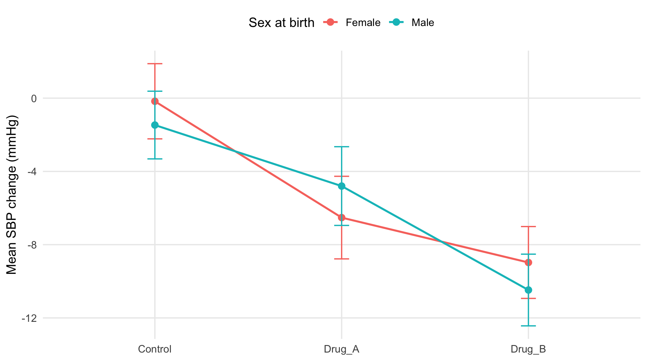
Figure 13.3: Mean SBP change by treatment arm and sex at birth.
Parallel lines suggest that treatment has a similar effect in females and males. Here, the lines cross, suggesting possible differences by sex, but the interaction test is not significant (\(p=0.23\)). Therefore, there is no clear evidence that the treatment effect differs by sex.
13.4.2 Additive factorial model
If the interaction is not scientifically important and the data do not support appreciable effect modification, an additive model is easier to interpret.
13.4.2.1 Two-factor models
The linear-model syntax generalizes directly:
sbp_additive <- lm(sbp_change~treatment_arm+sex_at_birth, data=sbp_cc);
car::Anova(sbp_additive, type=2)
#> Anova Table (Type II tests)
#>
#> Response: sbp_change
#>               Sum Sq  Df F value             Pr(>F)
#> treatment_arm   4707   2   36.78 0.0000000000000032 ***
#> sex_at_birth      12   1    0.18               0.67
#> Residuals      22329 349
#> ---
#> Signif. codes:  0 '***' 0.001 '**' 0.01 '*' 0.05 '.' 0.1 ' ' 1
13.4.2.2 Three-factor model syntax
A full three-factor interaction model can consume many degrees of freedom and produce difficult-to-interpret estimates. It should be fitted because a three-way effect-modification question is scientifically motivated, not because three categorical columns happen to be present.
13.5 Unbalanced designs
Missing data can make group sizes unequal. When this happens, some ANOVA methods can give different results depending on the order in which treatment, sex, or other model terms are entered.
To avoid relying on term order, start with the scientific question and test that effect directly, such as the overall treatment effect or the treatment-by-sex interaction. Define the hypothesis first, then choose the model that matches it.