Exploratory data analysis (EDA) is the point at which the statistical problem becomes concrete. Before testing hypotheses, the analyst should know what each row represents, how variables are coded, where missing values occur, whether units are plausible, and how distributions differ across clinically relevant groups. EDA is therefore not a preliminary formality; it is part of model specification.
1.1 R essentials for a biomedical dataset
R is object-oriented in the practical sense that data, models, tables, and plots are stored as named objects and passed to functions. A compact working vocabulary is enough for most analyses:
| Task | Core R tools |
|---|---|
| inspect an object |
class(), str(), dplyr::glimpse()
|
| view dimensions |
nrow(), ncol(), dim()
|
| select variables | dplyr::select() |
| filter observations | dplyr::filter() |
| create variables | dplyr::mutate() |
| grouped summaries |
group_by() + summarise()
|
| reshape data |
pivot_longer(), pivot_wider()
|
| missingness |
is.na(), complete.cases(), drop_na()
|
| fit a model |
lm(), glm(), aov(), survival::coxph()
|
| inspect model output |
summary(), broom::tidy(), confint()
|
1.1.1 First look at the data
A few direct checks establish the data structure.
1.1.1.1 Dataset dimensions and variable names
dim(dat);
#> [1] 360  43
dplyr::glimpse(dat[, 1:12]);
#> Rows: 360
#> Columns: 12
#> $ patient_id        <chr> "P0003", "P0007", "P0008", "P0009", "P0010", "P0013", "P0015", "P0017", "P0018", "P0020", "P…
#> $ enrollment_date   <dttm> 2025-12-07, 2025-10-22, 2026-01-01, 2025-01-15, 2025-08-30, 2026-04-13, 2026-06-13, 2025-08…
#> $ site              <fct> Site_07, Site_02, Site_08, Site_04, Site_06, Site_03, Site_01, Site_08, Site_05, Site_07, Si…
#> $ region            <fct> West, North, West, South, East, South, North, West, East, West, North, West, North, North, W…
#> $ treatment_arm     <fct> Drug_B, Drug_A, Drug_A, Drug_A, Drug_A, Drug_B, Drug_A, Drug_A, Control, Control, Drug_B, Dr…
#> $ age_years         <dbl> 37, 39, 56, 65, 63, 49, 50, 52, 53, 59, 48, 59, 54, 41, 76, 60, 45, 51, 70, 57, 48, 67, 77, …
#> $ sex_at_birth      <fct> Female, Male, Male, Male, Male, Female, Female, Male, Male, Female, Male, Female, Male, Fema…
#> $ smoking_status    <fct> Former, Former, Current, Never, Current, Former, Former, Never, Never, Never, Never, Current…
#> $ baseline_severity <fct> Moderate, Moderate, Mild, Severe, Moderate, Moderate, Mild, Mild, Mild, Severe, Mild, Modera…
#> $ bmi_kg_m2         <dbl> 27.2, 30.7, 18.3, 31.8, 31.3, 34.7, 23.2, 18.0, 24.8, 28.5, 25.2, 27.2, 37.6, 29.3, 33.4, 33…
#> $ sbp_baseline_mmHg <dbl> 128.6, 111.0, 123.5, 134.0, 124.3, 144.4, 126.8, 124.2, 111.5, 143.9, 125.0, 138.2, 125.0, 1…
#> $ sbp_week12_mmHg   <dbl> 109.7, 109.2, 114.1, 126.8, 115.4, 142.3, 118.0, 119.0, 98.3, 147.6, 115.9, 122.6, 118.2, 11…
head(dat[, c("patient_id","treatment_arm","age_years","baseline_severity")], 4)
#> # A tibble: 4 × 4
#>   patient_id treatment_arm age_years baseline_severity
#>   <chr>      <fct>             <dbl> <fct>
#> 1 P0003      Drug_B               37 Moderate
#> 2 P0007      Drug_A               39 Moderate
#> 3 P0008      Drug_A               56 Mild
#> 4 P0009      Drug_A               65 Severe
1.1.2 Dataset audit
The current workbook contains one row per participant. Patient IDs should therefore be unique.
1.1.2.1 Structural integrity checks
audit <- tibble(metric=c("Participants","Variables","Unique patient IDs","Duplicate patient IDs","Missing cells"),
               value=c(nrow(dat), ncol(dat_raw), dplyr::n_distinct(dat$patient_id), sum(duplicated(dat$patient_id)), sum(is.na(dat_raw))))

kbl(audit, digits=0, caption="Dataset audit")| metric | value |
|---|---|
| Participants | 360 |
| Variables | 35 |
| Unique patient IDs | 360 |
| Duplicate patient IDs | 0 |
| Missing cells | 64 |
1.2 Variable types and analytical consequences
The distinction between continuous, discrete, categorical, binary, and ordinal data determines what summaries and models are meaningful.
| Data type | Definition | Examples in this workbook | Typical analytical consequence |
|---|---|---|---|
| Continuous | values on a quantitative scale where arithmetic differences are meaningful | age, BMI, SBP, CRP, biomarker, QoL | means/SDs or robust summaries; linear models when appropriate |
| Discrete/count | integer-valued event or counts |
ae_count_12w, hospital_days_90
|
count summaries; Poisson/negative-binomial models may be appropriate |
| Categorical | membership in one of a fixed set of nominal groups | treatment, site, region, smoking | frequencies/proportions; contingency tables or factor terms in models |
| Binary | categorical variable with two levels | response, adverse event, event observed | risks/proportions; binomial models; paired binary data need special methods |
| Ordinal | categories with a meaningful order | mild/moderate/severe baseline severity | preserve ordering; do not assume equal numeric spacing without justification |
The supplied data dictionary can be read directly from the workbook.
1.2.0.1 Variable roles and measurement scales
| Variable | Class | Role | Unit / Coding | Description | Intentional Missingness |
|---|---|---|---|---|---|
| patient_id | character | Identifier | P0001… | Synthetic patient identifier | No |
| enrollment_date | date | Time | YYYY-MM-DD | Enrollment date | No |
| site | categorical | Design | Site_01…Site_08 | Recruiting center | No |
| region | categorical | Design | North/South/East/West | Region of site | No |
| treatment_arm | categorical | Exposure | Control/Drug_A/Drug_B | Randomized treatment group | No |
| age_years | continuous | Covariate | years | Age at baseline | No |
| sex_at_birth | binary categorical | Covariate | Female/Male | Sex recorded at baseline | No |
| smoking_status | categorical | Covariate | Never/Former/Current | Smoking status | No |
| baseline_severity | ordinal | Covariate | Mild<Moderate<Severe | Baseline disease severity | No |
| bmi_kg_m2 | continuous | Covariate | kg/m^2 | Body mass index | No |
| sbp_baseline_mmHg | continuous | Baseline outcome | mmHg | Baseline systolic blood pressure | No |
| sbp_week12_mmHg | continuous | Follow-up outcome | mmHg | Week-12 systolic blood pressure | ~2.5% |
| dbp_baseline_mmHg | continuous | Covariate | mmHg | Baseline diastolic blood pressure | No |
| heart_rate_bpm | continuous | Covariate | beats/min | Baseline heart rate | No |
| hba1c_pct | continuous | Biomarker | % | Glycated hemoglobin | No |
| ldl_mg_dL | continuous | Biomarker | mg/dL | LDL cholesterol | ~2.5% |
| hdl_mg_dL | continuous | Biomarker | mg/dL | HDL cholesterol | No |
| creatinine_mg_dL | continuous | Biomarker | mg/dL | Serum creatinine | No |
| egfr_mL_min_1_73m2 | continuous | Biomarker | mL/min/1.73m^2 | Estimated glomerular filtration rate | No |
| wbc_10e9_L | continuous | Biomarker | 10^9/L | White blood cell count | No |
| crp_baseline_mg_L | continuous, skewed | Biomarker | mg/L | Baseline C-reactive protein | ~1.8% |
| crp_week12_mg_L | continuous, skewed | Follow-up biomarker | mg/L | Week-12 C-reactive protein | ~4.5% |
| biomarker_baseline_ng_mL | continuous | Primary continuous endpoint baseline | ng/mL | Synthetic inflammatory biomarker at baseline | No |
| biomarker_week12_ng_mL | continuous | Primary continuous endpoint follow-up | ng/mL | Synthetic inflammatory biomarker at week 12 | ~4% |
| adherence_pct | continuous | Process | 0-100% | Treatment adherence | No |
| qol_baseline_0_100 | continuous | Patient-reported outcome | 0-100 | Baseline quality-of-life score | No |
| qol_week12_0_100 | continuous | Patient-reported outcome | 0-100 | Week-12 quality-of-life score | ~3.5% |
| clinical_response_12w | binary | Primary binary endpoint | 0=No, 1=Yes | Clinical response at week 12 | No |
| adverse_event_12w | binary | Safety endpoint | 0=No, 1=Yes | Any adverse event by week 12 | No |
| ae_count_12w | discrete count | Safety endpoint | 0-6 events | Number of adverse events by week 12 | No |
| hospital_days_90 | discrete count | Utilization endpoint | days | Hospital days in first 90 days | No |
| followup_days | discrete | Time | days | Observed follow-up time | No |
| time_to_event_days | continuous/discrete time | Time-to-event | days | Time to clinical event or censoring | No |
| event_observed_90d | binary | Time-to-event endpoint | 0=Censored,1=Event | Clinical event observed within follow-up | No |
| sampling_weight | continuous | Sampling | relative weight | Educational sampling weight for weighted estimates | No |
1.2.1 Storage class versus scientific role
A variable’s storage class is not always identical to its scientific type. For example, a 0/1 endpoint can be stored as numeric yet remain binary for analysis. Likewise, disease severity can be stored as a factor with ordered labels; treating it as 1, 2, 3 in a regression imposes an equal-spacing assumption that may not be scientifically defensible. In this book it is generally modeled as a factor unless a proportional ordinal trend is explicitly intended.
1.3 Missing data
Missingness should be quantified before derived analyses are run. na.rm=TRUE is useful for descriptive statistics, but silently dropping different observations in different models can make results difficult to compare.
1.3.1 Quantify missingness
missing <- dat_raw |> summarise(across(everything(), ~sum(is.na(.x)))) |>
                      pivot_longer(everything(), names_to="variable", values_to="n_missing")

missing <- missing |> mutate(percent=100*n_missing/nrow(dat_raw)) |>
                      filter(n_missing>0) |> arrange(desc(percent))

kbl(missing, digits=2, caption="Variables with missing values")| variable | n_missing | percent |
|---|---|---|
| crp_week12_mg_L | 18 | 5.00 |
| qol_week12_0_100 | 13 | 3.61 |
| biomarker_week12_ng_mL | 11 | 3.06 |
| ldl_mg_dL | 9 | 2.50 |
| sbp_week12_mmHg | 7 | 1.94 |
| crp_baseline_mg_L | 6 | 1.67 |
1.3.1.1 Visual pattern of missingness
ggplot(missing, aes(percent, reorder(variable, percent))) +
  geom_col(width=.65, fill="#547D8E") +
  geom_text(aes(label=sprintf("%.1f%%", percent)), hjust=-.12, size=3.2) +
  scale_x_continuous(expand=expansion(mult=c(0,.18))) +
  labs(x="Missing observations (%)", y=NULL)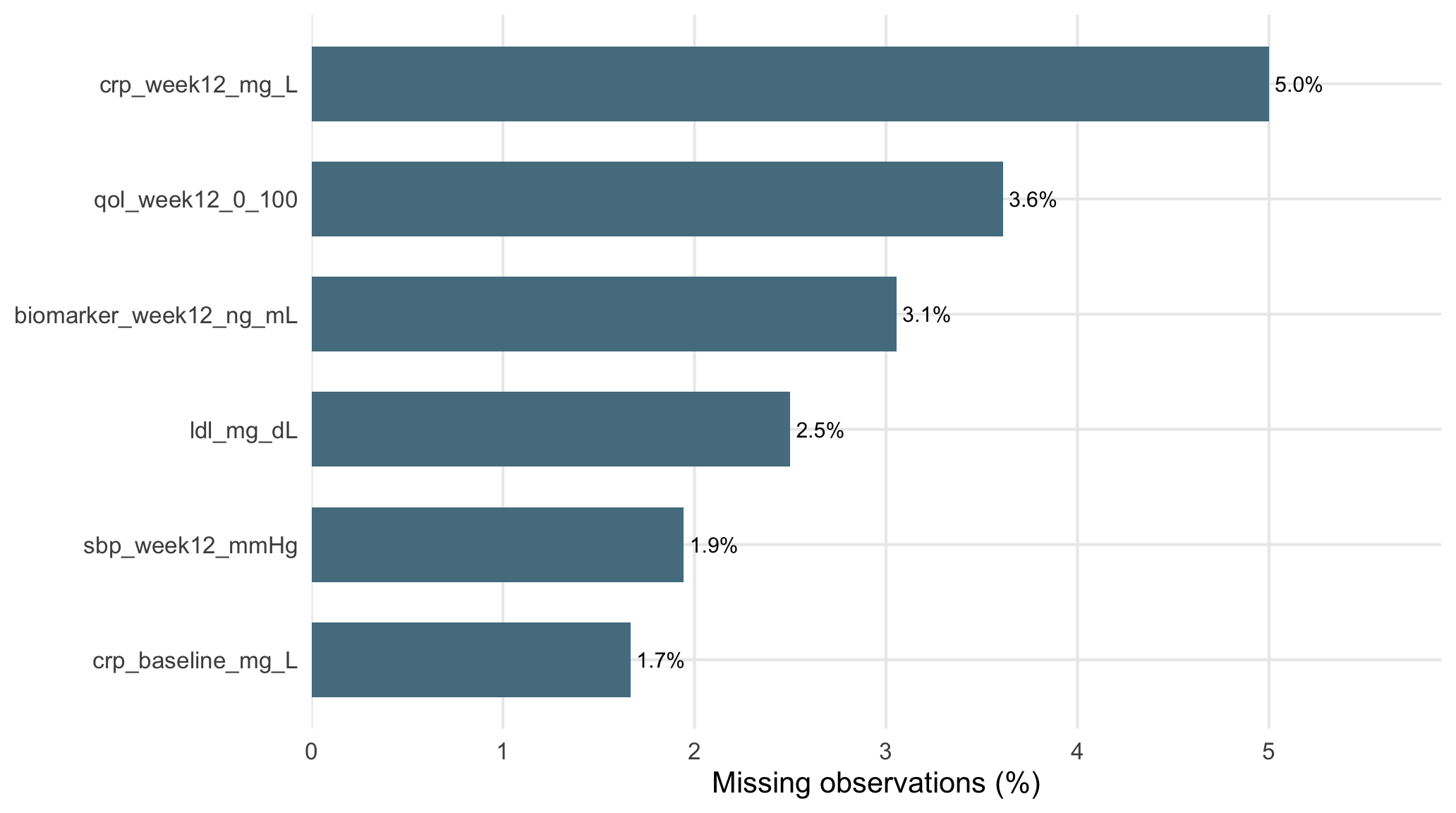
Figure 1.1: Percentage missing by variable.
1.3.2 Interpret the missingness mechanism
The missing percentages are small, but their mechanism is not specified. This distinction matters. A low percentage of missing values does not by itself prove that complete-case analysis is unbiased. In a real study, the analysis plan should consider why values are missing, whether missingness depends on observed or unobserved variables, and whether multiple imputation or other sensitivity analyses are required.
1.3.2.1 Filtering, selecting, and recoding
older <- dat |> filter(age_years>=65) |>
         dplyr::select(patient_id, treatment_arm, age_years, sbp_baseline_mmHg)

control_a <- dat |> filter(treatment_arm %in% c("Control","Drug_A")) |> droplevels()

highest_crp <- dat |> arrange(desc(crp_baseline_mg_L)) |>
               dplyr::select(patient_id, treatment_arm, crp_baseline_mg_L) |> head(6)

older; highest_crp
#> # A tibble: 81 × 4
#>    patient_id treatment_arm age_years sbp_baseline_mmHg
#>    <chr>      <fct>             <dbl>             <dbl>
#>  1 P0009      Drug_A               65              134
#>  2 P0029      Control              76              147.
#>  3 P0040      Control              70              129.
#>  4 P0045      Control              67              137.
#>  5 P0046      Drug_A               77              144.
#>  6 P0069      Drug_A               72              142.
#>  7 P0071      Drug_A               65              145
#>  8 P0083      Drug_B               66              140.
#>  9 P0091      Control              70              115.
#> 10 P0097      Drug_B               71              129.
#> # ℹ 71 more rows
#> # A tibble: 6 × 3
#>   patient_id treatment_arm crp_baseline_mg_L
#>   <chr>      <fct>                     <dbl>
#> 1 P0363      Control                    36.1
#> 2 P0465      Control                    23.0
#> 3 P0713      Drug_B                     20.4
#> 4 P0009      Drug_A                     17.5
#> 5 P0827      Control                    17.3
#> 6 P0708      Drug_B                     16.9
1.3.3 Derived change scores
The change variables represent the difference between the measurement at 12 weeks and the baseline measurement. A negative SBP change therefore indicates a decrease in blood pressure, whereas a positive SBP change indicates an increase.
\[ \Delta Y_i = Y_{i,12\text{wk}}-Y_{i,0}. \]