Multi-omics integration aims to combine multiple layers of molecular data, such as transcriptomics, proteomics, epigenomics, and metabolomics, from the same set of biological samples. One powerful approach for integrating multi-omics data is matrix factorization, a family of dimensionality reduction techniques designed to uncover hidden structures or patterns shared across different data types.
So, What Is Matrix Factorization?
Matrix factorization is a technique used to decompose a large, complex matrix into simpler, smaller matrices that are easier to analyze and interpret. The basic idea is to break down the data into underlying factors that explain the patterns or relationships observed in the original matrix.
Imagine you have a large matrix where columns represent samples, such as tumor or normal samples, and rows represent gene expression levels across samples. The matrix is essentially a snapshot of how genes behave across various conditions. However, this matrix is high-dimensional, making it difficult to directly interpret how different samples relate to each other based on the raw data.
Matrix factorization aims to reduce this high-dimensional data into a lower-dimensional space. This lower-dimensional space represents key factors that capture the major axes of variation in the data. Each latent factor can be thought of as a vector or axis in this reduced space.
The second matrix produced through matrix factorization is the activity matrix, which represents how much each sample contains of each factor. In other words, it reflects the activity of the factors.
When you multiply the latent factor matrix by the activity matrix, you get an approximation of the original matrix but with far fewer parameters. This allows you to uncover hidden patterns in the data.
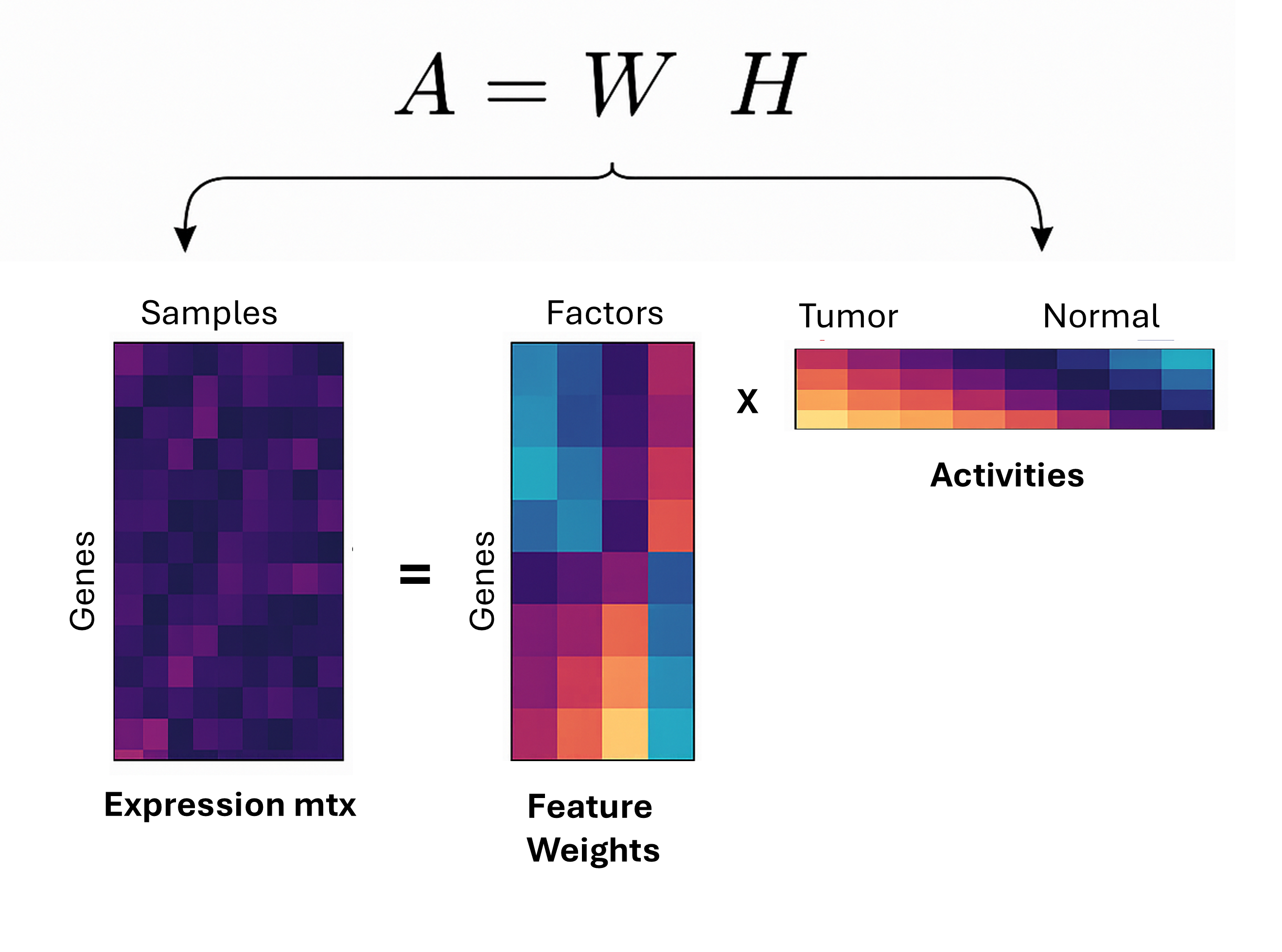
In the previous example, we have an expression matrix (A), which is decomposed into:
- Weight matrix (W): latent factors representing the major axes of variation in the data.
- Activity matrix (H): the activity or strength of each factor in each sample.
For instance, tumor samples might have a high activity score for a latent factor that represents genes involved in cell proliferation or immune evasion, reflecting the tumor’s biological processes. Normal samples, on the other hand, might have a low activity score for this same factor, reflecting that these biological processes are less active in normal tissue.
For the weight matrix (W), the higher the weight, the more important a gene is in contributing to the factor. In this way, the latent factors discovered through matrix factorization act like axes or vectors that define the main directions in the data where tumor and normal tissues vary.
In a more technical sense, these factors are linear combinations of the original gene expression features, meaning they reflect weighted combinations of genes that are most strongly associated with the biological differences between tumor and normal tissues.
By projecting samples onto these latent factors, you can gain a clearer understanding of how tumor and normal samples differ based on underlying, biologically meaningful axes. Matrix factorization reveals hidden structure in the data, allowing you to focus on the key factors driving variation. This can be used for downstream interpretation, biomarker discovery, or therapeutic target identification.